To use VLOOKUP in Excel, type =VLOOKUP(lookup_value, table_array, col_index_num, FALSE) in a cell, where the lookup value sits in the first column of the range and FALSE forces an exact match.
This guide walks through the formula step by step, then covers lookups between two sheets and two files, approximate matches, every common error and the modern alternatives XLOOKUP and INDEX/MATCH.
How to use VLOOKUP in Excel: Step-by-step
Picture a price list with part numbers in column A, names in column B and prices in column C, rows 2 to 20. You want the price for the part number typed in cell F2.
- Click the cell where the result should appear, for example G2.
- Type
=VLOOKUP(to start the formula. - Click F2, the cell holding the value you want to find, then type a comma.
- Select the range A2:C20, press F4 to make it absolute (
$A$2:$C$20), then type a comma. - Type
3, because price is the third column of the range counting from column A, then type a comma. - Type
FALSE)to ask for an exact match. - Press Enter. The full formula reads
=VLOOKUP(F2,$A$2:$C$20,3,FALSE)and the cell shows the price.
The absolute reference lets you drag the formula down to look up more part numbers without the table range shifting, even after adding multiple rows inside the table.
VLOOKUP methods compared
| Your situation | Use this | Why |
|---|---|---|
| Find one exact ID, name or code | VLOOKUP with FALSE | Returns a value only when the match is exact, otherwise #N/A |
| Grade bands, tax brackets, price tiers | VLOOKUP with TRUE on a sorted first column | Finds the closest value at or below the lookup value |
| Return column sits left of the lookup column | XLOOKUP or INDEX/MATCH | VLOOKUP can only return columns to the right of the first column |
| Microsoft 365 and a custom message when nothing matches | XLOOKUP | Exact match by default and an if_not_found argument |
| Workbook must open in Excel 2016 or 2019 | VLOOKUP or INDEX/MATCH | XLOOKUP is not available in Excel 2016 and Excel 2019 |
How does VLOOKUP work for dummies?
VLOOKUP reads down the first column of a range until it finds your value, then moves across that row to the column number you gave it. The V stands for vertical, because it searches down a column.
| Argument | What you put there | Example |
|---|---|---|
| lookup_value (required) | The value to find; it must be in the first column of table_array | F2 or "Fontana" |
| table_array (required) | The range holding both the lookup column and the return column | $A$2:$C$20 |
| col_index_num (required) | Which column to return, counting the left-most column of the range as 1 | 3 |
| range_lookup (optional) | FALSE or 0 for an exact match, TRUE or 1 for an approximate match | FALSE |
Why is VLOOKUP so confusing at first?
| Sticking point | What is actually happening |
|---|---|
| The column number | It counts from the first column of your range, not from column A of the sheet. In B2:D11, column B is 1. |
| The lookup column must be first | VLOOKUP only searches the left-most column of table_array and returns columns to its right, so you may need to move rows or columns in Excel first. |
| The fourth argument is optional | Leaving it out means TRUE, an approximate match, which is rarely what a beginner wants. |
| Copied formulas break | A relative range such as A2:C20 slides down as you fill; absolute $A$2:$C$20 stays put. |
| Numbers that look identical do not match | A number stored as text in one column and as a number in the other is not an exact match. |
The “dangerous default” warning
Always type FALSE (or 0) as the fourth argument unless you deliberately want an approximate match. When range_lookup is left out, Excel uses TRUE. On an unsorted first column, an approximate match can return a value from the wrong row with no error at all, so a wrong price or name looks perfectly valid.
When to use approximate match (TRUE)
Approximate match suits ranges: commission bands, shipping tiers or letter grades. VLOOKUP returns the row with the largest value that is less than or equal to your lookup value.
- Put the lower bound of each band in the first column, for example 0, 60, 70, 80, 90.
- Put the result for each band in the next column, for example F, D, C, B, A.
- Select the first column and sort it smallest to largest with Data > Sort A to Z.
- Type
=VLOOKUP(B2,$E$2:$F$6,2,TRUE)where B2 holds the score. - Press Enter. A score of 85 returns B, because 80 is the largest bound not above 85.
A lookup value smaller than the smallest value in the first column returns #N/A, so start the bands at the lowest possible value.
How to use VLOOKUP in Excel between 2 sheets
The table can sit on another tab of the same workbook. Excel writes the sheet name into the reference for you. If that tab is locked, unprotect the workbook before you edit the source table.
- On the sheet that needs the result, click the result cell and type
=VLOOKUP(. - Click the lookup value cell on the current sheet, then type a comma.
- Click the other sheet's tab at the bottom of the window and select the table range.
- Press F4 to make the range absolute, then type a comma.
- Type the column number, a comma and
FALSE), then press Enter. - Confirm the formula looks like
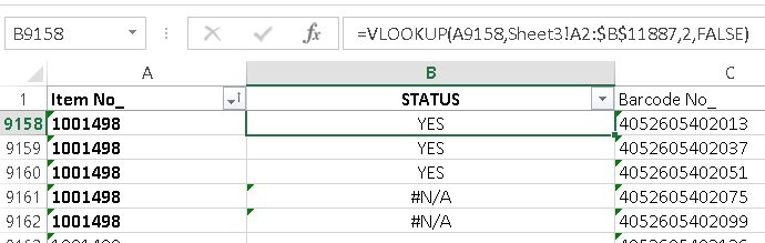
=VLOOKUP(A2,'Client Details'!$A:$F,3,FALSE), with the sheet name in quotes when it contains a space.
How to use VLOOKUP in Excel between 2 files
- Open both workbooks.
- In the workbook that needs the result, click the result cell and type
=VLOOKUP(. - Click the lookup value cell, then type a comma.
- Switch to the other workbook with View > Switch Windows and select the table range.
- Type a comma, the column number, a comma and
FALSE), then press Enter. - Save both files. Excel stores a link to the source workbook and may ask to update it the next time you open the file.
Alternative ways to look up data
| Function | Formula shape | Best for |
|---|---|---|
| XLOOKUP | =XLOOKUP(F2,A2:A20,C2:C20) | Microsoft 365: any direction, exact match by default, custom not-found text |
| INDEX/MATCH | =INDEX(C2:C20,MATCH(F2,A2:A20,0)) | Every Excel version, including return columns to the left |
| HLOOKUP | =HLOOKUP(F1,A1:T3,3,FALSE) | Tables laid out in rows instead of columns |
| FILTER | =FILTER(A2:C20,A2:A20=F2) | Returning every matching row, not only the first one |
Are there any alternatives to VLOOKUP, such as INDEX/MATCH or XLOOKUP?
| Question | VLOOKUP | XLOOKUP | INDEX/MATCH |
|---|---|---|---|
| Default match type | Approximate (TRUE) | Exact | Set by MATCH; 0 is exact |
| Return a column left of the lookup column | No | Yes | Yes |
| Breaks when you insert a column | Yes, the column number stays fixed | No, it uses ranges | No, it uses ranges |
| Custom text when nothing is found | Needs IFERROR or IFNA | Built in with if_not_found | Needs IFERROR or IFNA |
| Works in Excel 2016 and 2019 | Yes | No | Yes |
Tips for reliable VLOOKUP results
| Do this | Why |
|---|---|
| Lock the range with $ signs | The formula keeps looking at the same table when filled down |
| Store numbers and dates as numbers, not text | Text-formatted numbers can return wrong or unexpected values |
| Sort the first column when using TRUE | Approximate match assumes a sorted first column |
| Use ? and * wildcards with FALSE | =VLOOKUP("Fontan?",B2:E7,2,FALSE) matches any final letter; type ~ before a real ? or * |
| Clean stray spaces with TRIM or CLEAN | Leading or trailing spaces and nonprinting characters stop exact matches |
| Use a named range or an Excel table for table_array | The reference reads clearly and grows with the data |
If a lookup column has repeated values, it helps to remove duplicates from the column first, because VLOOKUP returns only the first match.
Test a VLOOKUP formula returns the right row
- Pick one lookup value and find its row in the table by eye.
- Compare that row's value in the target column with the formula result.
- Change the lookup value to one that does not exist; an exact-match formula should show #N/A.
- Click the result cell and select Formulas > Evaluate Formula to step through each argument.
- Drag the formula down a few rows and confirm the table range still shows the same $ references.
Troubleshooting common VLOOKUP errors
#N/A in the cell
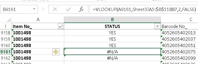
With FALSE the exact value is not in the first column; with TRUE the value is smaller than the smallest entry.
- Check that the value exists in the first column of table_array.
- Remove extra spaces with
=TRIM()on both sides. - Wrap the formula as
=IFNA(VLOOKUP(...),"Not found")to show a message instead.
#REF! in the cell
col_index_num is larger than the number of columns in table_array.
- Count the columns in the range starting at 1.
- Lower the column number or widen the range to include the return column.
#VALUE! in the cell
col_index_num is less than 1.
- Change the third argument to 1 or higher.
#NAME? in the cell
Text in the formula is missing quotation marks, or the function name is misspelled.
- Put text lookup values in quotes, as in
=VLOOKUP("Fontana",B2:E7,2,FALSE). - Check the spelling of VLOOKUP.
#SPILL! in the cell
The lookup value is a whole column such as A:A, so Excel tries to return many results.
- Refer to one cell instead:
=VLOOKUP(A2,A:C,2,FALSE). - Or anchor the column with the @ operator:
=VLOOKUP(@A:A,A:C,2,FALSE).
Still not working?
VLOOKUP returns a wrong value with no error
range_lookup is TRUE or left out and the first column is not sorted.
- Add
FALSEas the fourth argument. - Or sort the first column smallest to largest if you need an approximate match.
VLOOKUP fails to match values that look the same
One column stores numbers as text, or cells contain curly quotes or nonprinting characters.
- Select the column and convert it with Data > Text to Columns > Finish, or use
=VALUE(). - Run
=CLEAN()and=TRIM()on the lookup column.
Results go wrong after copying the formula down
The table range is relative and shifted with each row.
- Edit the formula and press F4 on the range to add $ signs.
- Fill the formula down again.
Results go wrong after inserting a column
col_index_num is a fixed number and now points at a different column.
- Update the column number.
- Or switch to XLOOKUP or INDEX/MATCH, which refer to ranges.
Frequently asked questions
Why do we use VLOOKUP in Excel?
VLOOKUP finds a value in the first column of a table and returns a related value from the same row. It saves you from searching manually, for example pulling a price from a part number or a name from an employee ID across thousands of rows.
What is VLOOKUP in Excel and how do you use it?
VLOOKUP is a lookup function that searches a column vertically. Type =VLOOKUP(lookup_value, table_array, col_index_num, FALSE), where the lookup value is in the first column of the range and the column number counts from that first column.
How do I use VLOOKUP in Excel to match values in two columns?
Use VLOOKUP with FALSE against the second column: =VLOOKUP(A2,$C$2:$C$100,1,FALSE). A value that appears in both columns is returned, and #N/A marks values that exist only in the first column.
How do I use VLOOKUP between two tabs?
Start the formula on one tab, then click the other tab and select the table range while typing. Excel adds the sheet name, such as 'Client Details'!A:F, to the reference automatically.
Can I use VLOOKUP between two Excel files?
Yes. Open both workbooks, start the formula in one, and select the table range in the other. Excel stores the source workbook path in the formula and may prompt to update links when you reopen the file.
Can I use XLOOKUP in Excel 2016?
No. Microsoft states XLOOKUP is not available in Excel 2016 or Excel 2019. A workbook built in a newer version with XLOOKUP can be opened there, but use VLOOKUP or INDEX/MATCH for formulas that must work in those versions.
What is the difference between VLOOKUP and HLOOKUP?
VLOOKUP searches down the first column of a table and returns a value from a column to the right. HLOOKUP searches across the first row and returns a value from a row below it.
Why does my VLOOKUP return #N/A when the value exists?
The most common causes are extra spaces, numbers stored as text, or a lookup value that is not in the first column of the range. Clean the data with TRIM and check the range starts at the lookup column.