How to Hide Chart Series with No Data in Excel (4 Easy Methods)

To hide a chart series with no data in Excel, hide or filter out its source row, because Excel does not plot data in hidden rows and columns by default.

This guide covers the four methods that do it: filtering, formulas with NA(), conditional formatting plus a VBA macro, and dynamic named ranges. It also covers the Hidden and Empty Cells settings that control what the chart does, and fixes for when a series will not disappear.

The fastest way to hide an empty series: Chart Filters

If you only need one chart cleaned up once, Chart Filters is the quickest route. It hides the series and its legend entry without touching any cells.

1. Click the chart to select it.
2. Select the Chart Filters button next to the upper-right corner of the chart.
3. On the Values tab, clear the check box for each series that has no data.
4. Select Apply.

Chart Filters is manual: when a hidden series gets data later, you have to tick it again yourself. For a chart that should hide empty series on its own, use the filter method below.

Which of the 4 methods fits your chart?

All four methods keep your data in the workbook. They differ in whether they update on their own and whether they hide the whole series or only its empty points.

Your situation	Use this method	What it hides	Updates on its own?
Each series sits in its own row and some rows are empty	1. Filter out rows where a count column is 0	The whole series, legend entry included	After you reapply the filter
Series have some blanks that plot as zero or break the line	2. Formulas that return NA() for missing values	Empty points; an all-empty series draws nothing	Yes, formulas recalculate
You refresh the same report often and want one click	3. Conditional formatting to flag empty rows, plus a VBA macro to hide them	The whole series, legend entry included	Each time you run the macro
Data fills in over time, such as months not yet reached	4. Dynamic named ranges built with OFFSET	Empty trailing points at the end of each series	Yes, the names resize as data arrives

1. How to Hide Series with No Data Using the Filter Method

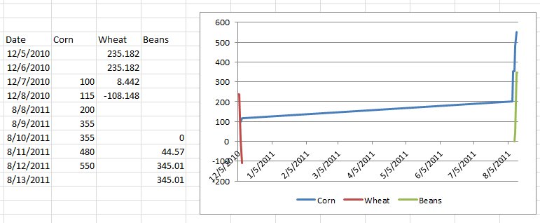
This method works when each chart series comes from one worksheet row. A helper column counts the numbers in each row, and AutoFilter hides the rows that count zero. Hidden rows drop out of the chart, so the empty series and its legend entry disappear.

1. Add a column to the right of your chart data and give it the header Count.
2. In the first data row of that column, enter =COUNT(B2:M2), adjusting the range to cover that row's values, and fill it down to the last series.
3. Click any cell in the data and select Data > Filter.
4. Open the filter arrow on the Count column and clear the check box for 0.
5. Select OK. Rows with no numbers are hidden, and their series leave the chart.
6. When new data arrives, select Data > Reapply so rows that now have values come back.

If your series run down columns instead of across rows, AutoFilter cannot hide them. Hide the empty column instead: right-click its letter and choose Hide, and the chart drops that series the same way.

2. Dynamic Hiding of Series with No Data Using Formulas

Formulas cannot delete a series, but they control what each point plots. Microsoft's guidance for missing information is to mark it with #N/A, and the NA() function returns that value.

Build the chart from a helper block of formulas instead of the raw data. Empty cells then return #N/A, and the chart has nothing to plot for them.

1. Copy your series names into a spare area of the sheet, for example column P, with the category labels above them in row 1.
2. Next to the first name, enter =IF(B2="",NA(),B2) and fill it across and down so the helper block mirrors your data.
3. Right-click the chart, choose Select Data, and set Chart data range to the helper block.
4. Select OK. Points with no data no longer plot as zero, and a series with no data at all draws no bars, lines or markers.
5. To drop the empty series' legend entry too, add the Count column from Method 1 to the helper block and filter out the rows showing 0.

In line, scatter and radar charts, Excel connects the line across #N/A points by default. The Show #N/A as an empty cell option under Hidden and Empty Cells leaves a gap instead, but Microsoft lists it as a Microsoft 365 Insiders feature, so your version may not have it.

3. Hiding Series in Your Chart by Using Conditional Formatting or VBA

Conditional formatting changes how cells look; it cannot hide a chart series. Use it to flag the empty rows, then let a short macro hide those rows so the chart drops them.

Macros need the Developer tab, which Excel hides by default. Turn it on from File > Options > Customize Ribbon by ticking Developer under Main Tabs.

1. Select the series rows, for example A2:M10, and choose Home > Conditional Formatting > New Rule.
2. Choose Use a formula to determine which cells to format, enter =COUNT($B2:$M2)=0, pick a fill color, and select OK. Empty series rows are now highlighted.
3. On the Developer tab, select Record Macro, keep the name Macro1, select OK, and then select Stop Recording.
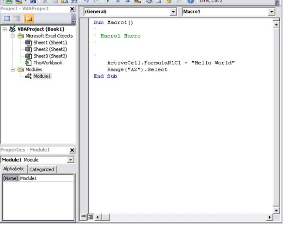
4. Select Macros, choose Macro1, and select Edit to open the Visual Basic Editor.
5. Replace the recorded code with the macro below, changing the sheet name and range to match your data.
6. Close the editor, then select Macros > Macro1 > Run. Every row with no numbers is hidden and its series leaves the chart.
7. Save the file as an Excel Macro-Enabled Workbook, because a standard workbook cannot keep macro code.

The macro code for step 5 is in the next section.

The VBA macro that hides empty series rows

Paste this over the recorded code in the Visual Basic Editor. Change Sheet1 and B2:M10 to your sheet name and the range that holds the series values.

Sub Macro1()
    Dim rw As Range
    For Each rw In Worksheets("Sheet1").Range("B2:M10").Rows
        rw.EntireRow.Hidden = (Application.WorksheetFunction.Count(rw) = 0)
    Next rw
End Sub

The macro checks each row of the range. A row with no numbers gets its entire row hidden, and a row with at least one number is unhidden, so a series that gains data comes back the next time you run it.

You should see: Rows with no numbers disappear from the sheet, and their series and legend entries leave the chart.

Office disables macros by default when you open a macro-enabled file, so enable content only in workbooks you trust.

4. Using Named Ranges and Dynamic Data Series to Exclude No Data Series

Microsoft documents a way to make a chart range resize itself with defined names built on OFFSET. The chart then plots only the rows that hold numbers, so months or periods with no data yet stay off the chart.

The steps assume labels in column A, values in column B, and a header in row 1.

1. On the Formulas tab, in the Defined Names group, select Define Name.
2. In Name, type Sales. In Refers to, enter =OFFSET($B$2,0,0,COUNT($B:$B),1) and select OK.
3. Select Define Name again. Name it Date and enter =OFFSET($A$2,0,0,COUNT($B:$B),1), so the labels stop where the values stop.
4. Right-click the chart and choose Select Data.
5. Under Legend Entries (Series), select the series and choose Edit. In Series values, enter =Sheet1!Sales and select OK.
6. Under Horizontal (Category) Axis Labels, select Edit, enter =Sheet1!Date, and select OK twice.
7. Type a value in the next empty row of column B. The chart extends to include it.

Use COUNT for a column of numbers and COUNTA for a column of text. OFFSET needs a positive height, so a name cannot shrink to nothing; a series with no data at all still needs Method 1 or Method 3 to leave the chart.

How to check the empty series are really gone

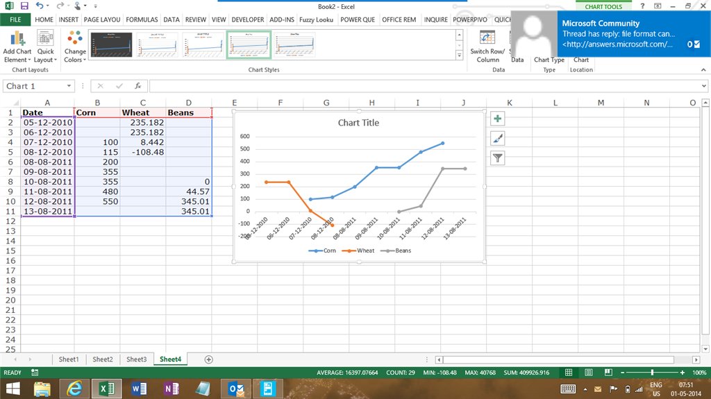
A hidden series should vanish from the plot area and the legend while its source cells remain in the workbook.

1. Look at the legend. Series with no data should not be listed.
2. Look at the row numbers beside your data. Filtered or hidden rows show as a gap in the numbering, which confirms Method 1 or Method 3 ran.
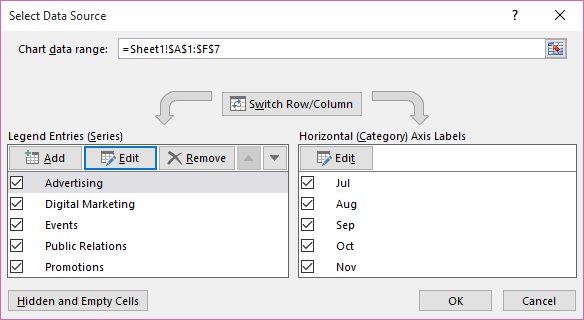
3. Right-click the chart, choose Select Data, and confirm the empty series still appear under Legend Entries (Series). That shows they are hidden, not removed.
4. Type a number into one empty series row, then reapply the filter or rerun the macro. The series should return to the chart.
5. For Method 4, select Formulas > Name Manager and confirm Sales and Date refer to the OFFSET formulas.

Change how the chart treats hidden and empty cells

Every method above relies on one chart setting: by default, Excel does not plot data in hidden rows and columns, and it shows empty cells as gaps. Check it if a hidden series still shows up.

1. Click the chart.
2. On the Chart Design tab (Design under Chart Tools in older versions), select Select Data.
3. Select Hidden and Empty Cells.
4. Clear Show data in hidden rows and columns so hidden series stay off the chart.
5. Under Show empty cells as, choose Gaps, Zero or Connect data points with line.
6. Select OK, then OK again.

On a scatter chart that shows only markers, empty cells can display as gaps or zero, but not as a connecting line.

Fix a chart series that will not hide

Find the symptom that matches your chart and follow only the steps under it.

The empty series is still in the chart after you hide its row

The chart has Show data in hidden rows and columns turned on, so it plots hidden rows anyway.

1. Right-click the chart and choose Select Data.
2. Select Hidden and Empty Cells.
3. Clear Show data in hidden rows and columns.
4. Select OK twice.

You want to hide the data on the sheet but still show it in the chart

Hiding rows removes their data from the chart by default, which is the opposite of what you need here.

1. Right-click the chart and choose Select Data > Hidden and Empty Cells.
2. Check Show data in hidden rows and columns.
3. Select OK twice, then hide the rows. The chart keeps plotting them.

A series you hid cannot be shown again with Chart Filters

The series was deleted with Remove in Select Data, and a removed series no longer appears in Chart Filters.

1. Press Ctrl + Z if the removal was your last action.
2. Otherwise, right-click the chart and choose Select Data.
3. Under Legend Entries (Series), select Add, pick the series name and value cells, and select OK twice.

A series still shows in the legend even though it plots nothing

Formulas that return #N/A stop the points from plotting, but the series itself stays in the chart.

1. Add the Count column from Method 1 next to the helper block.
2. Filter out the rows where Count is 0, or run the Method 3 macro on that range.
3. Confirm the legend entry is gone.

Additional Tips for Effective Chart Management

Hidden series are still data in the file. These points prevent the usual surprises when a chart hides things on its own.

Tip	Why it matters
Hide series instead of removing them	A series deleted with Remove in Select Data cannot be brought back with Chart Filters, and editing series can break links to the source data
Keep the Count helper column next to the data	It shows at a glance which series are empty and drives both the filter and the conditional formatting rule
Reapply the filter after each data update	AutoFilter does not re-evaluate on its own, so a series that gains data stays hidden until you select Reapply
Size OFFSET names with COUNT on the value column	Counting the labels instead would keep empty periods on the axis when labels are filled in ahead of the data
Share macro workbooks with care	Office disables macros by default, so other people must enable content before the Method 3 macro runs
Leave a note near filtered data	Gaps in the row numbers are easy to miss, and the next editor may not know why a series is missing

Frequently Asked Questions

How do you hide chart series with no data in Excel automatically?

Add a column that counts each series row with =COUNT(), turn on Data > Filter, and filter out rows where the count is 0. Hidden rows are not plotted by default, so empty series leave the chart. Select Data > Reapply after new data arrives.

How do you hide a series in an Excel chart without deleting it?

Select the chart, select the Chart Filters button, clear the series on the Values tab, and select Apply. The series and its cells stay in the workbook, and ticking the box again brings it back. Avoid Remove in Select Data, which deletes it.

Can you hide data in Excel but still show it in the chart?

Yes. Right-click the chart, choose Select Data > Hidden and Empty Cells, and check Show data in hidden rows and columns. You can then hide the source rows or columns while the chart keeps plotting their values.

How do you hide an axis in an Excel chart?

Click the chart, open the chart design tab, select Add Chart Element > Axes, and click the axis type to turn it off. To hide only the tick marks or labels, format the axis and set Axis labels to None.

How do you hide a chart in Excel?

Open the Selection pane with Home > Find & Select > Selection Pane, or press Alt + F10. Select the hide icon next to the chart. The chart stays in the file, and the same pane shows it again.

How do you hide the chart title in Excel?

Click the chart, select the + button at its top-right corner, and clear the check box next to Chart Title. Ticking the box again restores the title. The same steps work for charts in Word, PowerPoint and Outlook.

How do you hide the chart title in Word?

Charts in Word use the same chart tools as Excel. Click the chart, select the + button at its top-right corner, and clear Chart Title. Ticking the box again brings the title back.

How do you hide the legend in an Excel chart?

Click the legend to select it and press Delete. To bring it back, select the chart, select the + button at the top-right, point to Legend, and choose where it should appear.

How do you hide the chart title and legend together?

Select the chart, select the + button at its top-right corner, and clear both Chart Title and Legend. Both elements disappear in one pass, and ticking the boxes restores them.

Why does an empty series still show in my chart legend?

A series with no values is still part of the chart, so Excel keeps its legend entry even though nothing plots. Clearing it in Chart Filters, or hiding its source row with the default Hidden and Empty Cells settings, removes it from the chart completely.