How to Hide Chart Data in Excel – 6 Steps

To hide chart data in Excel, select the chart, select the Chart Filters button, clear the series or categories you want gone on the Values tab, and select Apply.

The data stays in your worksheet, so you can bring it back at any time. This guide also covers hiding source rows and columns, making a series invisible, hiding worksheet values while the chart still shows them, and what to do when a chart goes blank.

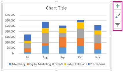
Hide chart data with Chart Filters in 6 steps

Chart Filters hide a series or a category from the chart without touching a single cell. It is the fastest way to hide specific data points, and it is fully reversible.

1. Click the chart to select it.
2. Select the Chart Filters button next to the upper-right corner of the chart.
3. Open the Values tab.
4. Clear the check box for each data series you want to hide.
5. Clear the check box for each category, such as a month or region, you want to hide.
6. Select Apply.

The chart redraws without the cleared items. To show them again, reopen Chart Filters, tick the boxes and select Apply.

Which way to hide chart data fits your case?

Each route hides something different: the chart item, the worksheet cells, or both. Match your goal to a row before you change anything.

Your goal	Use this	What stays visible	Easy to undo?
Hide one series or a few categories from the chart only	Chart Filters > Values tab	All worksheet cells	Yes, tick the box again
Hide the same rows from both the sheet and the chart	Hide the source rows or columns	Nothing from those rows	Yes, Unhide
Keep a series in the chart's structure but make it invisible	Format the series with No Fill and No Outline	Legend entry and worksheet cells	Yes, reapply a fill or outline
Hide worksheet numbers but keep the chart showing them	Custom number format ;;; plus Show data in hidden rows and columns if you also hide rows	The chart	Yes, set the format back to General
Switch data in and out of the chart with a flag you control	A helper column with AutoFilter	Rows that match the filter	Yes, clear the filter
Remove a series for good	Select Data > Remove	Worksheet cells only	Only with Ctrl + Z; Chart Filters cannot show it again

Use the hidden rows and columns method

By default, Excel does not plot data in hidden rows and columns. Hiding the source rows therefore removes those points from the chart and from view on the sheet.

1. Select the row numbers or column letters that hold the data you want to hide. Hold Ctrl to add nonadjacent rows or columns.
2. Right-click the selection.
3. Select Hide.
4. Check the chart. The hidden rows or columns no longer appear in it.
5. To bring them back, select the rows or columns on both sides of the hidden ones, right-click, and select Unhide.

A double line between two row numbers or column letters marks where data is hidden. Double-click that line to unhide it quickly.

Format data points to have no visibility

This keeps the series in the chart, including its legend entry, but paints it invisible. Use it when you need a placeholder series or want the axis scale to stay the same.

1. Click the series once to select every point in it. Click a single point a second time to select only that point.
2. Open the Format tab on the ribbon.
3. In the Shape Styles group, select Shape Fill and then No Fill.
4. Select Shape Outline and then No Outline.
5. For a line series, No Outline is what hides the line itself.
6. Press Ctrl + Z straight away if you formatted the wrong element.

Right-clicking the series and choosing Format Data Series opens the Format pane, which holds the same fill and line options. To show the series again, reapply a fill color or outline.

Use custom number formatting to make data invisible

This is the answer when you want to hide data but still show the chart. The ;;; format blanks the cells on screen, while the values stay in place and the chart keeps plotting them.

1. Select the cells whose values you want to hide.
2. On the Home tab, select the Number Format button next to Number to open Format Cells.
3. In the Category box, select Custom.
4. In the Type box, enter ;;; (three semicolons).
5. Select OK. The cells look empty, but the chart is unchanged.

The hidden values still show in the formula bar when you select a cell. To display them again, open the same dialog and pick General or another number format.

Use a helper column to control what the chart shows

A helper column turns hiding into a switch. AutoFilter hides the rows you filter out, and the chart skips hidden rows, so changing one flag updates the chart.

1. Add a column next to your chart data and name it Show.
2. Type Yes in each row the chart should plot and No in each row it should hide.
3. Click any cell in the data and select Data > Filter.
4. Open the filter arrow on the Show column and clear the check box for No.
5. Select OK. The filtered rows are hidden and drop out of the chart.
6. To show everything again, open the same arrow and select Clear Filter from "Show", or turn off Data > Filter.

Change a row's flag from Yes to No, then reapply the filter to hide it. Filtering only conceals rows, so every value stays in the sheet.

Hide rows but keep them in the chart

Sometimes you want the opposite: tidy up the sheet by hiding rows, but keep the chart complete. One chart setting controls this, and it is off by default.

1. Click the chart.
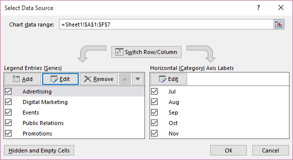
2. On the Chart Design tab (Design under Chart Tools in older versions), in the Data group, select Select Data. You can also right-click the chart and choose Select Data.
3. Select Hidden and Empty Cells.
4. Check Show data in hidden rows and columns.
5. Optionally, under Show empty cells as, pick Gaps, Zero or Connect data points with line.
6. Select OK, then OK again to close Select Data Source.

The same dialog has a Show #N/A as an empty cell option, but Microsoft lists it as a Microsoft 365 Insiders feature, so it may be missing from your version.

How to check the data is hidden, not deleted

A hidden item should vanish from the chart while its numbers still exist somewhere you can reach.

1. Reopen Chart Filters and confirm the hidden items are listed with cleared check boxes. A removed series cannot be restored from there.
2. Right-click the chart, select Select Data, and confirm the series still appears under Legend Entries (Series).
3. On the sheet, look for a double line between row numbers or column letters if you hid source rows or columns.
4. Select a cell formatted with ;;; and confirm its value shows in the formula bar.

Understand chart behavior with hidden or filtered data

Excel treats each kind of hiding differently when it draws a chart. This table shows what the chart does in each case with default settings.

What you did	What the chart does	Setting that changes it
Hid rows or columns	Skips those points	Show data in hidden rows and columns
Filtered rows with AutoFilter	Skips the filtered-out rows, because filtering hides them	Show data in hidden rows and columns
Cleared a series or category in Chart Filters	Hides it; the cells are untouched	Tick it again in Chart Filters
Left cells empty	Shows a gap	Show empty cells as: Gaps, Zero or Connect data points with line
Applied the ;;; number format	Plots the values as normal	None needed; the format affects the sheet only
Removed a series in Select Data	Deletes the series from the chart	Add it back with Add in Select Data Source

On scatter charts that show only markers, empty cells can display as gaps or zero, but not as a connecting line.

Fix chart data that hides or shows when it should not

Find the symptom that matches your chart and run only the fix under it.

The chart disappears or goes blank when data is hidden

Excel does not plot hidden rows and columns by default, so hiding or filtering all the source rows leaves nothing to draw.

1. Click the chart and select Chart Design > Select Data.
2. Select Hidden and Empty Cells.
3. Check Show data in hidden rows and columns.
4. Select OK twice. The chart plots the hidden rows again while they stay hidden on the sheet.

A series hidden earlier cannot be shown with Chart Filters

The series was removed in Select Data instead of hidden, and a removed series no longer appears in Chart Filters.

1. Press Ctrl + Z if the removal was your last action.
2. Otherwise, right-click the chart and select Select Data.
3. Under Legend Entries (Series), select Add.
4. Select the original name and value cells for the series, then select OK twice.

Hidden worksheet data still shows in the chart

The chart has Show data in hidden rows and columns turned on, or the cells were blanked with a number format rather than hidden.

1. Right-click the chart and select Select Data.
2. Select Hidden and Empty Cells and clear Show data in hidden rows and columns.
3. Select OK twice.
4. If the cells use the ;;; format, hide the rows instead, or use Chart Filters to hide the series.

Hidden values reappear when someone selects a cell

The ;;; format hides values only on the grid; the formula bar still shows them.

1. Treat ;;; as a display choice, not protection.
2. Move sensitive source data to a separate worksheet you control, or leave it out of any copy you share.

Additional tips and best practices

Hidden data is still data. Keep these points in mind before you share a workbook with a chart that hides anything.

Tip	Why it matters
Back up the workbook before removing any series	Remove in Select Data deletes the series, and changes there can break links to the source data
Prefer Chart Filters over Remove	Filtered items come back with one tick; removed series do not
Be mindful of hidden data in large workbooks	Hidden rows, ;;; cells and filtered-out series stay in the file and travel with every copy you send
Check the Hidden and Empty Cells setting before you hide rows	Whether hidden rows stay in the chart depends on Show data in hidden rows and columns, which is off by default
Leave a note next to hidden data	Double lines between row numbers are easy to miss, and the next editor may not know why a chart looks short

Frequently asked questions

How do you hide data in an Excel graph?

Click the graph, select the Chart Filters button beside it, clear the series or categories you want hidden on the Values tab, and select Apply. The worksheet data is untouched, and ticking the boxes again restores the hidden items.

Can you hide data in Excel but still show it in the chart?

Yes. Apply the custom number format ;;; to blank the cells while the chart keeps plotting them. If you hide the rows instead, open Select Data > Hidden and Empty Cells and check Show data in hidden rows and columns so the chart still includes them.

Does hiding chart data delete it?

No. Chart Filters, hidden rows, No Fill formatting and the ;;; format all leave the cells and values in the workbook. Only Remove in the Select Data Source dialog deletes a series from the chart, and Chart Filters cannot show that series again.

Why does my Excel chart disappear when I hide rows?

Excel does not plot data in hidden rows and columns by default. Right-click the chart, select Select Data > Hidden and Empty Cells, and check Show data in hidden rows and columns to keep the chart intact while the rows stay hidden.

How do you hide a chart in Excel?

Open the Selection pane with Home > Find & Select > Selection Pane, or press Alt + F10. Select the chart in the list and select its hide icon. The chart stays in the file but is no longer visible on the sheet.

How do you find a hidden chart in Excel?

Press Alt + F10 to open the Selection pane, which lists every object on the sheet, including hidden ones. Select the unhide icon next to the chart to show it again. Hidden objects are easy to forget, so check this pane when a chart seems missing.

How do you hide the chart title in Excel?

Click the chart, select the + button at its top-right corner, and clear the check box next to Chart Title. The same steps work in Word, PowerPoint and Outlook charts, and ticking the box again brings the title back.

How do you hide the chart data table in PowerPoint?

Select the chart, select the + button at its top-right corner, and clear the Data Table check box. PowerPoint charts use the same chart tools as Excel, so the same steps hide a data table in an Excel chart.

How do you hide data labels on a chart in Word?

Charts in Word use the same tools as Excel. Select the chart, then choose Add Chart Element > Data Labels > None on the chart design tab. You can also right-click a data label and select Delete, or select it and press Delete.

How do you hide a single data point in an Excel chart?

Click the series once, then click the point again so only it is selected. On the Format tab, set Shape Fill to No Fill and Shape Outline to No Outline. The point becomes invisible while its value stays in the worksheet.

How do you show hidden data in an Excel chart again?

Reverse the method you used. Tick the items again in Chart Filters, unhide the source rows or columns, reapply a fill to a No Fill series, or check Show data in hidden rows and columns under Select Data > Hidden and Empty Cells.