To perform multiple linear regression in Excel, load the Analysis ToolPak, select Data Analysis on the Data tab, choose Regression and give it one Y column plus several X columns, or type =LINEST(y_range, x_range, TRUE, TRUE) in a cell.
This guide covers both methods in desktop Excel for Windows and Mac, how to read R², F and the coefficients, a worked example with real numbers, and fixes for the errors people hit most.
Method 1: Using Excel's Data Analysis Toolpak
The Regression tool in the Analysis ToolPak fits a least-squares line through your data and writes a full output table. It analyzes how one dependent variable is affected by one or more independent variables, and it uses the LINEST worksheet function underneath.
Arrange the data first: one column for the outcome (Y) and one column per predictor (X), with the X columns side by side and a header in the first row.
- In Excel for Windows, select File > Options > Add-Ins. In Excel for Mac, go to Tools > Excel Add-ins instead.
- In the Manage box, select Excel Add-ins, then select Go.
- Check Analysis ToolPak and select OK. If Excel says it is not installed, select Yes to install it.
- Go to the Data tab and select Data Analysis in the Analysis group.
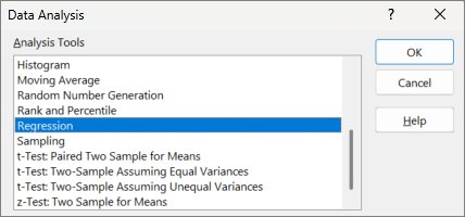
- Select Regression in the list and select OK.
- In the Y range box, select the outcome column including its header. In the X range box, select all the predictor columns as one block, including headers.
- Turn on the labels option so Excel uses your headers as variable names, choose where the output goes, and select OK.
Excel writes a summary block with R², a variance (ANOVA) table with the F statistic, and a coefficient table with one row for the intercept and one row per predictor. Each row lists the coefficient, its standard error, a t statistic and a p-value.
Which method should you use?
| Your situation | Use this | Why |
|---|---|---|
| You want a one-off report with every statistic labelled | Method 1: Regression tool | Writes a labelled output table, plus optional residual output and charts |
| Your data changes and results should update by themselves | Method 2: LINEST | A formula recalculates; the Regression tool output is static and must be re-run |
| You use Excel for the web | Neither in the browser; select Open in Desktop | Excel for the web has no Regression tool and cannot run meaningful LINEST regression |
| You need a prediction from the fitted model in another formula | Method 2: LINEST with INDEX or TREND | The coefficients are live values you can reference directly |
| You are new to regression | Method 1: Regression tool | Labelled rows make the output easier to read than a bare array |
Prerequisites for Performing Multiple Linear Regression in Excel
| Requirement | Detail |
|---|---|
| Desktop Excel | Excel for Windows or Excel for Mac. Excel for the web can display regression results but cannot create them. |
| Analysis ToolPak (Method 1 only) | A free add-in that ships with Excel; load it once from Excel Add-ins. |
| One dependent variable | A single column (or single row) of Y values. LINEST requires Y to be one row or one column when there are several X variables. |
| Two or more independent variables | Each predictor in its own column, all with the same number of rows as Y. |
| Numeric data only | Text categories must be converted to 0/1 indicator columns before you run the model. |
| More rows than predictors | Degrees of freedom are n – k – 1, so with k predictors you need comfortably more than k + 1 observations for useful F and t tests. |
| One worksheet | Analysis ToolPak tools run on one worksheet at a time; grouped sheets get results only on the first sheet. |
Method 2: Using Excel Formulas (LINEST Function)
LINEST calculates the least-squares line y = m1x1 + m2x2 + ... + b and returns the coefficients as an array. Its syntax is LINEST(known_y's, [known_x's], [const], [stats]).
Set const to TRUE to calculate the intercept normally, or FALSE to force it to zero. Set stats to TRUE to get the full block of regression statistics.
- Put Y in one column and the predictors in adjacent columns, for example Y in E2:E12 and four predictors in A2:D12.
- Select an empty cell with at least five free rows below it and one free column per predictor plus one to its right.
- Type
=LINEST(E2:E12,A2:D12,TRUE,TRUE)and press Enter. In Excel for Microsoft 365 the result spills into a 5-row block. - In older Excel without dynamic arrays, first select the whole output range (5 rows by k + 1 columns), type the formula, then press Ctrl + Shift + Enter.
- Read the first row right to left: the last value is the intercept b, the one before it is the coefficient for the first X column, and so on.
- To pull out one value, wrap the formula in INDEX, for example
=INDEX(LINEST(E2:E12,A2:D12,TRUE,TRUE),3,1)for R².
The coefficients come back in reverse column order, {mn, mn-1, ..., m1, b}. Forgetting this is the most common way to misread LINEST.
How to read the regression output
With stats set to TRUE, LINEST returns five rows. The Regression tool reports the same statistics with labels.
| LINEST row | Columns contain | What it tells you |
|---|---|---|
| Row 1 | Coefficients mn … m1, then intercept b | The change in Y for a one-unit change in each X, holding the others fixed |
| Row 2 | Standard errors sen … se1, then seb | How precise each coefficient is; divide a coefficient by its standard error to get its t statistic |
| Row 3 | r2, then sey | r2 is the share of Y's variation the model explains (0 to 1); sey is the standard error of the Y estimate |
| Row 4 | F, then df | F tests whether the whole model beats chance; df is n – k – 1 when the intercept is calculated |
| Row 5 | ssreg, then ssresid | Regression and residual sums of squares; r2 equals ssreg / (ssreg + ssresid) |
To confirm the model is useful, compare F with the critical F value, or run =F.DIST.RT(F, v1, v2) where v1 = n – df – 1 and v2 = df. A result below 0.05 means the relationship is unlikely to be chance. For one predictor, =T.DIST.2T(ABS(t), df) gives its two-tailed p-value.
Understanding Multiple Linear Regression
Multiple linear regression estimates one outcome from two or more predictors with the equation y = m1x1 + m2x2 + ... + mnxn + b. Each m is the effect of its own predictor while the others stay constant, and b is the intercept.
| Term | Meaning | Example |
|---|---|---|
| Dependent variable (y) | The value you want to explain or predict | Assessed value of an office building |
| Independent variables (x1 … xn) | The predictors | Floor space, offices, entrances, age |
| Coefficient (m) | Change in y per one-unit change in that x, others held constant | Value drops by about $234 per extra year of age |
| Intercept (b) | Predicted y when every x is zero | Often has no practical meaning on its own |
| Least squares | The fitting rule: choose m and b so the sum of squared residuals is as small as possible | Used by both the Regression tool and LINEST |
| Residual | Actual y minus predicted y for one row | Large residuals flag rows the model fits badly |
Use it instead of simple regression when one predictor alone leaves too much unexplained, or when you need each factor's effect with the others accounted for.
Practical Example: Real-World Data Application
Microsoft's own LINEST documentation uses 11 office buildings to predict assessed value from floor space (x1), offices (x2), entrances (x3) and building age (x4). Paste the data at cell A1 and enter =LINEST(E2:E12,A2:D12,TRUE,TRUE) in A19 to reproduce the results.
| Floor space (x1) | Offices (x2) | Entrances (x3) | Age (x4) | Assessed value (y) |
|---|---|---|---|---|
| 2310 | 2 | 2 | 20 | $142,000 |
| 2333 | 2 | 2 | 12 | $144,000 |
| 2356 | 3 | 1.5 | 33 | $151,000 |
| 2379 | 3 | 2 | 43 | $150,000 |
| 2402 | 2 | 3 | 53 | $139,000 |
| 2425 | 4 | 2 | 23 | $169,000 |
| 2448 | 2 | 1.5 | 99 | $126,000 |
| 2471 | 2 | 2 | 34 | $142,900 |
| 2494 | 3 | 3 | 23 | $163,000 |
| 2517 | 4 | 4 | 55 | $169,000 |
| 2540 | 2 | 3 | 22 | $149,000 |
The first output column reads -234.24 (age coefficient), 13.268 (its standard error), 0.99675 (r2), 459.75 (F) and 1,732,393,319 (ssreg), with df = 6. An r2 of 0.997 means the four predictors explain almost all the variation in value.
With v1 = 11 – 6 – 1 = 4 and v2 = 6, the critical F at alpha 0.05 is 4.53, and 459.75 is far above it. The age coefficient's t value is -234.24 / 13.268 = -17.7, well beyond the two-tailed critical value of 2.447, so age is a significant predictor.
Additional Tips and Best Practices
| Tip | Why it matters |
|---|---|
| Check model assumptions with residuals | Plot actual against predicted values (TREND returns the fitted values); a pattern in the residuals means a straight-line model is the wrong shape. |
| Handle categorical variables with 0/1 columns | Use one indicator column fewer than the number of categories. A full set duplicates the intercept, and LINEST drops the redundant column. |
| Watch for collinearity | Predictors that are combinations of each other add nothing. LINEST shows a removed column as a 0 coefficient with a 0 standard error. |
| Do not predict far outside your data | Predicted values may not be valid outside the range of values used to fit the equation. |
| Keep the data in one contiguous block | Gaps or text in the ranges break both tools; if you need room for new observations, insert several rows at once inside the block. |
| Use model evaluation statistics together | Read r2, F and each t statistic; a high r2 alone does not prove every predictor is useful. |
| Prefer dynamic array formulas | Microsoft recommends dynamic arrays over legacy Ctrl+Shift+Enter formulas for new workbooks. |
Fix common regression errors in Excel
Data Analysis is missing from the Data tab
The Analysis ToolPak add-in is not loaded.
- Select File > Options > Add-Ins.
- Choose Excel Add-ins in the Manage box and select Go.
- Check Analysis ToolPak and select OK. If it is not listed, select Browse to locate it.
There is no Regression tool in Excel for the web
Excel for the web can view regression results but cannot create them, and it does not support the array entry LINEST needs.
- Select Open in Desktop to open the workbook in the Excel app.
- Run Method 1 or Method 2 there, then save; the results stay visible in the browser.
LINEST returns only one number or a #SPILL! error
In older Excel the output range was not selected first; in Microsoft 365 something blocks the spill area.
- In Microsoft 365, clear any data in the 5-row block below and to the right of the formula cell.
- In older Excel, select the full output range, type the formula and press Ctrl + Shift + Enter.
A coefficient and its standard error both show 0
LINEST found that column redundant (collinear) and removed it from the model.
- Check whether that X column is a sum or multiple of other X columns.
- For category indicators, delete one of the 0/1 columns and run the formula again.
Results only appear on the first sheet
Analysis ToolPak tools run on one worksheet at a time, and the sheets were grouped.
- Ungroup the sheets by selecting a single sheet tab.
- Run the Regression tool separately on each sheet.
Frequently Asked Questions
How do you perform multiple linear regression in Excel?
Load the Analysis ToolPak, select Data Analysis on the Data tab, choose Regression, and enter one Y range plus a block of X columns. Alternatively, type =LINEST(y_range, x_range, TRUE, TRUE) to get the coefficients and statistics as a formula that updates with the data.
What is multiple linear regression?
Multiple linear regression is a method that predicts one outcome from two or more predictors using y = m1x1 + m2x2 + … + b. Each coefficient shows how much y changes when its predictor rises by one unit while the other predictors stay the same.
Why use a multiple linear regression model?
Use multiple linear regression when an outcome depends on several factors at once. It separates each factor's effect from the others, tells you how much of the variation the factors explain together, and lets you predict new values, such as a building's value from its size, offices and age.
How do you interpret multiple linear regression results?
Start with r2 for overall fit, then check F against its critical value to confirm the model beats chance. Next read each coefficient: its sign gives direction and its size gives the effect per unit. Divide a coefficient by its standard error; a large absolute t value means that predictor matters.
How do you calculate multiple linear regression by hand?
The coefficients come from least squares: they minimize the sum of squared differences between actual and predicted y. With several predictors this needs matrix algebra, which is why Excel's LINEST function or the Regression tool is the practical route. Both use the same least-squares method.
What order does LINEST return the coefficients in?
LINEST returns coefficients in reverse order of the X columns, followed by the intercept: {mn, mn-1, …, m1, b}. With predictors in columns A to D, the first value belongs to column D and the fifth value is the intercept.
Can Excel for the web do multiple linear regression?
No. Excel for the web can show regression results but has no Regression tool, and it does not support the array-formula entry that meaningful LINEST regression requires. Open the workbook in the desktop app with Open in Desktop to run the analysis.
How do you include a categorical variable in Excel regression?
Convert the category to 0/1 indicator columns, using one column fewer than the number of categories. Including every category duplicates the intercept, and LINEST will drop the redundant column, showing it with a 0 coefficient and 0 standard error.
Conclusion
Use the Analysis ToolPak Regression tool for a labelled one-time report, and LINEST when results must update with the data or feed other formulas. Both run the same least-squares calculation, so the choice is only about static, labelled output versus a live formula.