How to add a drop down list in Excel: A step-by-step guide

To add a drop down list in Excel, select the cell, go to Data > Data Validation, choose List in the Allow box, then select your items or type them, separated by commas, in Source.

This guide covers Excel for Windows, Mac and the web, then editing, copying, removing and fixing a drop down list, building a dependent list, and adding a drop down in Word.

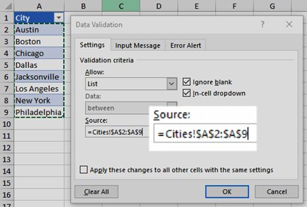
Step by step tutorial: Adding a drop down list in Excel

Keep the items in an Excel table. Any drop down based on a table updates itself when you add or remove items, so you never have to touch the rule again.

1. Type the items for the list in one column, one item per cell, for example on a sheet named Lists.
2. Select any cell in that list and press Ctrl + T to turn it into an Excel table, then select OK.
3. Select the cell where the drop down list should appear.
4. Go to the Data tab and select Data Validation.
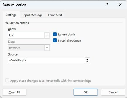
5. On the Settings tab, open the Allow box and select List.
6. Click in the Source box and select the list items, leaving out the header row.
7. Keep In-cell dropdown checked, and check Ignore blank if the cell may stay empty.
8. Select OK. An arrow appears beside the cell when you select it, and clicking the arrow shows your items.

Leave the header out of the selection, or it becomes one of the choices. To apply the same list to a whole column, select all of those cells in step 3 before opening Data Validation.

How to add a drop down in Excel with options

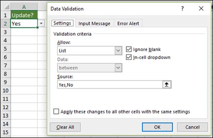
For a short fixed set such as Yes, No and Maybe, type the options straight into the Source box. No list on a worksheet is needed.

1. Select the cell or cells that need the drop down.
2. Go to Data > Data Validation.
3. On the Settings tab, set Allow to List.
4. In Source, type the options separated by commas with no spaces, for example Yes,No,Maybe.
5. Select OK, then click the arrow beside the cell to see the three options.

A typed list never updates on its own. To change the options later, reopen Data Validation and edit the Source text.

How to add a drop down list in Excel on Mac

1. Type the valid entries on a sheet in a single column or row, with no blank cells.
2. Select the cells where the drop down should appear.
3. On the Data tab, under Tools, select Data Validation or Validate.
4. Select the Settings tab, then choose List from the Allow pop-up menu.
5. Click in the Source box and select the list of entries on the sheet. The dialog shrinks so you can see the sheet.
6. Press Return or select Expand to restore the dialog, then select OK.

Excel for Mac also accepts values typed into Source with commas between them. If the validation command is unavailable, the sheet is protected or the workbook is shared.

How to add a drop down list in Excel online

1. On a worksheet, type the entries for the drop down, ideally in an Excel table.
2. Select the cell where the drop down should appear.
3. On the Data tab, select Data Tools > Data Validation.
4. On the Settings tab, set Allow to List.
5. In Source, select the list range, or type the entries separated by commas.
6. Check Ignore blank if people can leave the cell empty, and keep In-cell dropdown checked.
7. Select OK.

Excel for the web labels the message options differently: Show message on the Input Message tab, and Show Alert with a Type box on the Error Alert tab.

How to add an input message and error alert to a drop down list in Excel

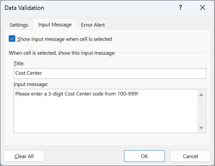
An input message tells people what to pick before they open the list. An error alert decides what happens when someone types a value that is not on it.

1. Select the cell with the drop down and open Data > Data Validation.
2. On the Input Message tab, check Show input message when cell is selected, then type a title and a message of up to 225 characters.
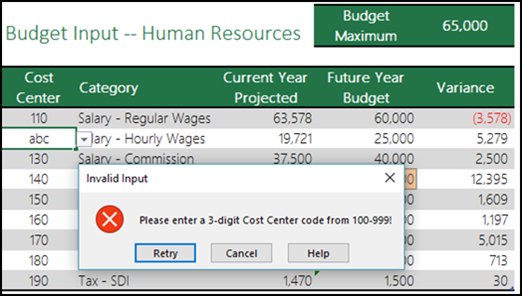
3. On the Error Alert tab, check Show error alert after invalid data is entered.
4. In Style, choose Stop to block any value that is not in the list, or Warning or Information to show a message but still allow it.
5. Type a title and message for the alert, then select OK.

If you leave the alert empty, Excel uses the title "Microsoft Excel" and the message "The value you entered is not valid. A user has restricted values that can be entered into this cell."

Tips for adding a drop down list in Excel

Tip	Why it helps
Turn the source list into a table first	Press Ctrl + T on the list, one of the Excel shortcut keys worth knowing, and new rows appear in the drop down automatically
Leave the header row out of Source	Only the cells you select become choices, so a header would show up as an option
Sort the source list before you build the drop down	People find items faster in alphabetical order; use Data > Sort A to Z on the source column, and remove duplicate entries so no choice appears twice
Widen the cell that holds the drop down	The width of the list is set by the width of that cell, so narrow cells cut entries short
Keep the source on its own sheet, then hide and protect it	People can pick from the list without seeing or changing the items behind it
Name the source range with Define Name	Source then reads =Departments instead of a cell address, which is easier to edit and to reuse elsewhere, for example as the lookup range in a VLOOKUP formula
Pick Stop as the error alert style	It is the only style that refuses values that are not in the list

Step by step tutorial on how to edit an Excel drop down list

How you edit a drop down depends on where its items come from. Select a cell with the drop down, open Data > Data Validation, and read the Source box on the Settings tab.

Excel supports four sources: a typed comma-separated list, a range of cells, a named range and an Excel table column.

List source	To add an item	To remove an item	Then update the rule?
Excel table	Type it in the row below the last item	Select it and press Delete; for an item mid-list, right-click it, select Delete, then OK to shift cells up	No. Every drop down based on the table updates automatically
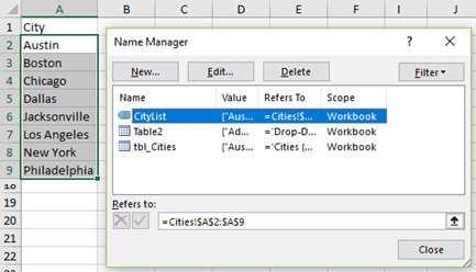
Named range	Type it at the end of the list	Delete the cell and shift cells up	Yes. Go to Formulas > Name Manager, select the name, reselect all the items in Refers to, then select Close and Yes
Range of cells	Type it at the end of the list	Delete the cell and shift cells up	Yes. Open Data > Data Validation and reselect the whole range in Source
Items typed in Source	Add it to the Source text after a comma	Delete it from the Source text	Editing the text is the update. Separate items with commas and no spaces

When you change Source, check Apply these changes to all other cells with the same settings so every cell that uses this drop down gets the new list.

Tips for editing an Excel drop down list

Tip	Why it helps
Check Source before you change anything	A list someone else built may be typed, a range, a named range or a table, and each is edited in a different place
Find an unknown range name in the Name Box	Select the source cells and the Name Box shows the name to look for in Name Manager
Delete mid-list items with Delete and Shift cells up	Clearing the cell instead leaves a blank gap in the middle of the drop down
Recheck the column width after adding longer items	The drop down is only as wide as its cell
Run Circle Invalid Data after removing items	Excel does not flag cells that still hold a value you removed; Data > Data Validation > Circle Invalid Data marks them
Unprotect the sheet or stop sharing the workbook first	Data Validation settings cannot be changed while the sheet is protected or the workbook is shared

How to create a dependent drop down list in Excel

A dependent, or cascading, drop down changes its items based on the choice in another cell, such as a Category cell that controls a Product cell. It combines named ranges with the INDIRECT function, which returns the range that a name typed in a cell refers to.

1. On a lists sheet, type each category's items in its own column, with the category name as the header, for example Fruit and Vegetables.
2. Select the items under the first header, without the header, then select Formulas > Define Name.
3. Type a name that matches the header exactly, such as Fruit, and select OK. Repeat for every category.
4. On the data sheet, select A2 and add a normal drop down whose Source is the row of category headers.
5. Select B2, open Data > Data Validation and set Allow to List.
6. In Source, type =INDIRECT(A2) and select OK.
7. Pick a category in A2, then open the drop down in B2. It lists only the items for that category.

Use category names that are also valid range names, such as single words like Fruit or Dairy. Copy A2:B2 down the column, and the relative reference in =INDIRECT(A2) follows each row.

How to copy a drop down list to another cell in Excel

A plain copy and paste brings the drop down along, because Ctrl + V pastes everything in the source cell, validation included. Use Paste Special when the target cells already hold values or formatting you want to keep.

1. Select the cell that has the drop down and press Ctrl + C.
2. Select the target cells, on the same worksheet or another one.
3. Select Home > Paste > Paste Special, or press Ctrl + Alt + V.
4. Select Validation, then select OK.

Paste Special with Validation pastes only the drop down rule. The values and formatting already in the target cells stay as they were.

How to find cells with a drop down list in Excel

Excel shows the drop down arrow only on the selected cell, so a sheet full of lists looks like plain cells. These steps reveal every one.

1. Open the worksheet you want to check.
2. On the Home tab, in the Editing group, select Find & Select > Data Validation. Excel selects every cell with a validation rule.
3. Or press Ctrl + G, select Special, select Data validation, then choose All for every rule or Same for cells that match the active cell.
4. Select one of the highlighted cells and look for the arrow at its right edge.
5. Open Data > Data Validation on that cell and read Source to see where its items come from.

How to remove a drop down list in Excel

1. Select the cell with the drop down. Hold Ctrl and click to add more cells.
2. Select Data > Data Validation.
3. On the Settings tab, select Clear All.
4. Select OK.

Clear All removes the rule, not the value already chosen in the cell. To clear every drop down on a sheet without hunting for them, press Ctrl + G, select Special > Data validation > All, then repeat the steps above.

How to add a drop down in Word

Word has no Data Validation. A drop down in a Word document is a content control, the same building block used to make a fillable form in Word, and it sits on the Developer tab, which stays hidden until you turn it on.

1. In Word, select File > Options > Customize Ribbon.
2. Under Main Tabs, check Developer and select OK.
3. Click where the drop down should go in the document.
4. Select Developer > Drop-Down List Content Control.
5. With the control selected, select Properties.
6. Under Drop-Down List Properties, select Add, type a choice in Display Name, such as Yes, and select OK.
7. Repeat step 6 for every choice, then select OK to close the properties.

Use Combo Box Content Control instead if people should also be able to type their own entry. Leave Contents cannot be edited unchecked, or nobody can pick a choice.

Excel drop down list not working

Data Validation is greyed out

A cell is still being edited, the sheet is protected, the workbook is shared, or the table is linked to a SharePoint site.

1. Press Enter or Esc to finish typing in the active cell.
2. Unprotect the worksheet, or stop sharing the workbook.
3. For a table linked to SharePoint, unlink it or convert it to a range, then open Data > Data Validation again.

The drop down arrow does not appear

In-cell dropdown is cleared on the Settings tab, or the cell is not selected.

1. Select the cell and open Data > Data Validation.
2. On the Settings tab, check In-cell dropdown and select OK.
3. Select the cell again; the arrow shows on the active cell only.

Values that are not in the list are accepted

The error alert style is Warning or Information, the alert is turned off, or the value was pasted or filled in, which skips the check.

1. On the Error Alert tab, check Show error alert after invalid data is entered and set Style to Stop.
2. Select Data > Data Validation > Circle Invalid Data to mark entries that slipped in.
3. To block drag-and-drop filling, go to File > Options > Advanced, clear Enable fill handle and cell drag-and-drop, then protect the worksheet.

New items do not show in the drop down

Source points at a fixed range or a named range that ends above the new items.

1. Convert the source list to a table with Ctrl + T and point Source at it.
2. Or update Source in Data Validation, or Refers to in Formulas > Name Manager, to include the new cells.

Entries are cut off in the drop down

The list is only as wide as the cell that holds it.

1. Drag the right border of the column header to widen the column.
2. Open the drop down again to check the longest entry fits.

Validation is ignored in some cells

Manual calculation is on, or the cell's formula returns an error such as #REF! or #DIV/0!.

1. Go to Formulas > Calculation Options and select Automatic.
2. Fix the formula error in the cell; Excel ignores validation there until it is fixed.

Excel drop down list FAQ

How do I add a drop down box in Excel?

A drop down box, drop down menu and drop down list are the same Excel feature. Select the cell, go to Data > Data Validation, set Allow to List, then select the items or type them separated by commas in Source and select OK.

How can I add to a drop down list in Excel?

If the list is an Excel table, type the new item below the last row and the drop down updates by itself. For a range or named range, add the item and then widen Source or Refers to. For a typed list, add it to the Source text.

How do I add a drop down in Excel with options?

Open Data > Data Validation, choose List under Allow, and type the options in Source separated by commas with no spaces, such as Yes,No,Maybe. Select OK and the options appear when you click the arrow beside the cell.

How do I add a drop down list to a cell in Excel?

Select the cell first, then go to Data > Data Validation, set Allow to List and fill in Source. To add it to many cells at once, select all of them before opening Data Validation, or copy the cell and paste with Paste Special > Validation.

Can I create a cascading drop-down list in Excel?

Yes. Give each set of child items a defined name that matches a category, add a category drop down in one cell, then use =INDIRECT(A2) as the Source of the second drop down. It shows only the items for the chosen category.

Is it possible to sort the items in a drop-down list?

Yes. The drop down shows items in the order of its source, so sort the source column with Data > Sort A to Z. For a typed list, rearrange the items in the Source box in the order you want them to appear.

How do I copy a drop-down list to another cell or worksheet?

Copy the cell with Ctrl + C, select the target cells on any sheet, then press Ctrl + Alt + V, choose Validation and select OK. This pastes only the drop down rule and keeps the values and formatting already in the target cells.

How do I edit an existing drop-down list?

Select a cell with the list and open Data > Data Validation to see its Source. Edit typed items there, reselect a range in Source, update a named range in Name Manager, or simply change the rows of an Excel table.

Can I add a drop down list in Word?

Yes. Turn on the Developer tab under File > Options > Customize Ribbon, then select Developer > Drop-Down List Content Control. Select Properties and use Add to type each choice. Word drop downs are content controls, not Data Validation.