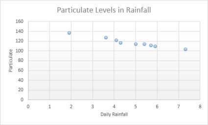
To change the X-axis range in an Excel chart, right-click the chart, choose Select Data, select Edit under Horizontal (Category) Axis Labels and pick a new cell range; in a scatter chart, set Minimum and Maximum in the Format Axis pane instead.
This guide covers every chart type, date axes, intervals, reversing the axis, resetting it, and the errors that stop the range from changing.
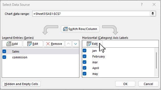
How to change the X-axis range in Excel with Select Data
Line, column, bar and area charts plot categories along the X-axis. Their range is the block of cells the chart reads, so you change it by pointing the axis at different cells.
- Right-click the chart and choose Select Data (Excel for Mac: Chart Design > Select Data).
- In the Select Data Source dialog, find the Horizontal (Category) Axis Labels box and select Edit.
- In Axis label range, select the new cells on the worksheet, for example A5:A16 instead of A2:A16.
- Select OK to close the axis labels box.
- Under Legend Entries (Series), select each series, choose Edit and shorten its values to the same rows.
- Select OK to apply the new X-axis range.
Keep the label range and the series values the same length, or Excel pads the axis with blank or numbered categories.
Understanding the X-axis in Excel charts
The X-axis is the horizontal axis. What "range" means depends on which of three axis types your chart uses.
| Axis type | Charts that use it | What sets its range |
|---|---|---|
| Category (text) axis | Line, column, bar, area, stock | The cells listed in Horizontal (Category) Axis Labels |
| Date axis | Line, column, bar, area, stock with date labels | The dates in the data, spaced in chronological order by a base unit of days, months or years |
| Value axis | XY (scatter) and bubble | Minimum and Maximum bounds in Format Axis |
| Not available | PivotChart reports | PivotCharts cannot use a date axis |
A category axis has fewer scaling options than a value axis. That is why the Minimum and Maximum boxes appear only for scatter and bubble charts.
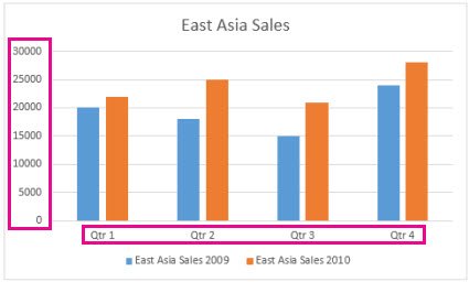
Methods to change the X-axis range in Excel charts
| What you want | Method | Works on |
|---|---|---|
| Plot a different block of rows | Select Data > Horizontal (Category) Axis Labels > Edit | Line, column, bar, area |
| Start the axis at 10 and stop at 50 | Format Axis > Minimum and Maximum | Scatter and bubble |
| Grow or shrink the plotted rows by dragging | Drag the corner of the highlighted source range | All charts built from a worksheet range |
| Hide a few categories without editing ranges | Chart Filters > Values tab | Most chart types |
| Space dates evenly by month or year | Axis Type > Date axis > Base unit | Line, column, bar, area, stock |
| Show fewer labels or flip the order | Interval between labels, Categories in reverse order | Category axes |
How to set X-axis minimum and maximum in an Excel scatter chart
XY (scatter) charts show values on both axes, so the horizontal axis takes numeric bounds just like the vertical one.
- Select the scatter chart to show the Chart Design and Format tabs.
- On the Format tab, open the Chart Elements box in the Current Selection group and choose the horizontal value axis.
- Select Format Selection to open the Format Axis pane.
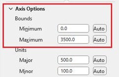
- Under Axis Options, type the start value in Minimum and the end value in Maximum.
- Set Major unit to control the gap between gridlines and labels.
- Select Reset next to a box to return it to Excel's automatic value.
Changing the bounds only changes what the chart shows; the data on the worksheet stays as it is.
How to change the X-axis range by resizing the chart data range
- Click the chart once; Excel highlights the source cells on the worksheet.
- Find the colour-coded ranges: one for the category axis labels, one for series names and one for the plotted values.
- Rest the pointer on the lower-right corner of the highlighted data.
- Drag up to remove rows from the X-axis, or down to add rows.
- Release the mouse; the chart redraws with the new range.
How to hide categories from the X-axis with chart filters
Filters hide chart data in Excel without editing any cell references, which narrows the X-axis for a quick view of one quarter or region.
- Select the chart.
- Select the Chart Filters button next to the chart.
- Open the Values tab.
- Clear the categories you want to drop from the X-axis.
- Select Apply.
- Tick the categories again later to bring them back.
On Windows you can also right-click the chart, choose Select Data and clear a category under Horizontal (Category) Axis Labels.
How to change the X-axis to a date axis in Excel
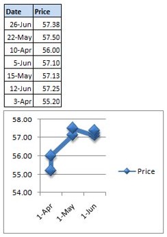
A date axis places dates in chronological order at fixed intervals, even when the worksheet rows are out of order. Excel picks it automatically for date labels, but you can switch it yourself.
- Right-click the horizontal axis and select Format Axis.
- In the Format Axis pane, select the Axis Options tab.
- Under Axis Type, select Date axis.
- Under Units, next to Base, select Days, Months or Years.
- Select Text axis instead if you want each row shown once with no gaps for missing dates.
A date axis is not possible when the dates are in the legend. Plot the data so the dates sit on the category axis first.
How to change X-axis interval and labels in Excel
- Select the chart, then on the Format tab choose Horizontal (Category) Axis in the Current Selection box.
- Select Format Selection.
- Under Tick Marks, set Interval between tick marks to the number of categories between ticks.
- Under Labels, choose Specify interval unit next to Interval between labels and type a number, such as 2 for every other label.
- Tick Categories in reverse order to flip the X-axis.
- Under Vertical axis crosses, choose At category number or At maximum category to move where the Y-axis meets it.
How to change X-axis labels in Excel without changing the data
Sometimes the range is right but the label text is wrong. Excel lets you type replacement labels directly, a different job from adding X-axis values to a chart.
- Right-click the X-axis labels and choose Select Data.
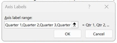
- Select Edit in the Horizontal (Category) Axis Labels box.
- In Axis label range, type the labels separated by commas, for example Quarter 1,Quarter 2,Quarter 3,Quarter 4.
- Select OK twice.
Typed labels no longer follow the worksheet, so edit the cells instead if the labels must update with the data.
How to reset the X-axis range in Excel to automatic
- On a scatter chart, open Format Axis and select Reset next to Minimum, Maximum and Major unit.
- On a category chart, open Select Data, select Edit under Horizontal (Category) Axis Labels and select the full original label column.
- Edit each series under Legend Entries (Series) back to the full value range.
- Under Axis Type, choose Automatically select based on data if you switched between text and date axes.
- Tick any categories you cleared under Chart Filters and select Apply.
Practical tips and best practices
| Tip | Why |
|---|---|
| Use a scatter chart when the X values are real numbers | Only value axes accept Minimum and Maximum bounds |
| Keep labels and series the same length | Mismatched ranges add blank or numbered categories |
| Prefer cell ranges over typed labels | Typed labels stop following the worksheet |
| Avoid zero or negative values on a logarithmic scale | Excel cannot draw a log scale through them |
| Use Chart Filters for a temporary view | No cell references change, so nothing breaks |
| Check links after editing series | Microsoft warns that changes may break links to the source data |
If blank rows still leave gaps on the axis, you can hide chart series with no data instead of trimming the range by hand.
Troubleshooting common issues with the Excel X-axis range
No Minimum or Maximum boxes for the X-axis
Line, column and bar charts use a category axis, which has no numeric bounds.
- Change the plotted rows with Select Data instead.
- Or select the chart, choose Change Chart Type on the Chart Design tab and pick X Y (Scatter).
- Open Format Axis again; Minimum and Maximum now appear.
X-axis shows 1, 2, 3 instead of your labels
Excel plotted your X column as a data series, or the axis label range is empty.
- Right-click the chart and choose Select Data.
- Remove the X column from Legend Entries (Series) if it appears there.
- Select Edit under Horizontal (Category) Axis Labels and select the label cells.
Dates on the X-axis show gaps or extra dates
A date axis spaces dates evenly and fills days with no data.
- Right-click the axis and select Format Axis.
- Under Axis Type, select Text axis.
- Or keep Date axis and change Base to Months or Years.
Chart stops updating after you change the range
Typed labels or edited series no longer link to the worksheet cells.
- Open Select Data and check each series and the axis label range.
- Replace typed values with cell references.
- Select OK.
Logarithmic scale will not apply
A logarithmic scale cannot be used for zero or negative values.
- Remove zero or negative X values from the plotted range.
- Or clear Logarithmic scale and use Minimum and Maximum instead.
Excel chart X-axis range FAQ
How do I change the X-axis range in Excel?
Right-click the chart, choose Select Data, select Edit under Horizontal (Category) Axis Labels and pick the new cells, then shorten each series to match. In a scatter chart, open Format Axis and type new Minimum and Maximum values instead.
Why can't I set the X-axis minimum and maximum in Excel?
Line, column, bar and area charts use a category axis, which has no Minimum or Maximum boxes. Only value axes have bounds, so switch to an XY (scatter) chart if your X values are numbers you want to scale.
How do I change where the X-axis starts in Excel?
In a scatter chart, type the start value in the Minimum box of the Format Axis pane. In a category chart, edit the axis label range in Select Data so it begins at the first row you want plotted.
How do I show only certain dates on the X-axis?
Use the Chart Filters button, open the Values tab, clear the dates you do not want and select Apply. To space dates by month or year instead, set Axis Type to Date axis and change the Base unit.
How do I reverse the X-axis in Excel?
Open Format Axis for the horizontal axis and tick Categories in reverse order. On a scatter chart the horizontal axis is a value axis, so the equivalent box is Values in reverse order.
How do I change the X-axis interval in Excel?
On a category axis, set Interval between tick marks, and under Labels choose Specify interval unit and type a number. On a scatter chart, change Major unit in the Format Axis pane to set the gap between labels.
Can I change the X-axis range in Excel for Mac?
Yes. Select the chart, choose Select Data on the Chart Design tab and edit the axis label range, or open Format Axis to set bounds on a scatter chart. Microsoft's axis settings apply to Excel for Mac as well as Windows.
How do I reset the X-axis range to automatic?
In Format Axis, select Reset next to Minimum and Maximum on a scatter chart. On a category chart, reselect the full original label and value ranges in Select Data, and set Axis Type back to Automatically select based on data.
Should you use a scatter chart for a custom X-axis range in Excel?
Use Select Data for text or date categories, and switch to an XY (scatter) chart only when the X values are numbers you need to start and stop at exact points. Category axes take their range from cells and have no bounds, while scatter charts treat the X-axis as a value axis with Minimum, Maximum and Major unit boxes. Picking the chart type that matches the data saves fighting the Format Axis pane.