How to find mean, median, and mode on Excel: 3 easy methods

To find the mean, median and mode in Excel, type =AVERAGE(A2:A11), =MEDIAN(A2:A11) and =MODE.SNGL(A2:A11) into three empty cells, replacing A2:A11 with your own range.

This guide covers those three functions, the Analysis ToolPak report, a manual sort-and-count method, a chart of the results, and fixes for #N/A, #SPILL! and a missing Data Analysis button.

Mean, median and mode formulas in Excel

The example below uses ten test scores in cells A2 to A11: 72, 85, 90, 85, 64, 78, 85, 90, 70 and 81. Type them in, or point the formulas at your own column.

1. Click an empty cell, type =AVERAGE(A2:A11) and press Enter. The mean of the sample scores is 80.
2. Click the next empty cell, type =MEDIAN(A2:A11) and press Enter. The median is 83, the midpoint between 81 and 85.
3. Click a third empty cell, type =MODE.SNGL(A2:A11) and press Enter. The mode is 85, because it appears three times.
4. Add a label such as Mean, Median and Mode in the cells to the left, so the results stay readable when you share the sheet.

The formulas recalculate as soon as you change any value in the range, so the three results always match the data.

Understanding the basics: mean, median, and mode

All three are measures of central tendency, the location of the centre of a group of numbers. In a symmetrical set they match; in a skewed set they drift apart, which is why reports often show all three.

Measure	What it is	Excel function	Example: 2, 3, 3, 5, 7, 10
Mean	The sum of the values divided by how many values there are	AVERAGE	30 / 6 = 5
Median	The middle value: half the numbers are above it, half below	MEDIAN	4 (midway between 3 and 5)
Mode	The value that occurs most often	MODE.SNGL or MODE.MULT	3
Range	The largest value minus the smallest value	MAX minus MIN	10 – 2 = 8

Use the median when a few extreme values pull the mean up or down, such as house prices or salaries. Use the mode for the most common size, score or answer.

Which Excel method to use for mean, median and mode

Your situation	Use this	Why
Results must update when the data changes	Method 1: AVERAGE, MEDIAN and MODE.SNGL	Formulas recalculate on every edit
You want a full statistics report in one pass	Method 2: Analysis ToolPak Descriptive Statistics	One dialog produces mean, median, mode and spread measures together
You are learning the maths or checking a result by hand	Method 3: sort and count	You see the middle value and each value's frequency directly
The data has two or more equally common values	MODE.MULT inside Method 1	MODE.SNGL returns only the first mode it finds

Preparing your data for analysis in Excel

AVERAGE, MEDIAN and both MODE functions ignore text, logical values and empty cells inside a referenced range, but they include cells that contain zero. Clean data before you calculate, or the results will be wrong without any error showing.

1. Put each value in its own cell in a single column, with one header in the first row.
2. Delete placeholder zeros for missing entries and leave those cells blank, because a zero counts as a real value.
3. Select the column, press Ctrl + 1, and on the Number tab choose General or Number under Category so the values are stored as numbers.
4. Look for numbers that start with an apostrophe or align to the left; those are stored as text and the functions skip them.
5. Remove error values such as #DIV/0! from the range, because an error inside the arguments makes the result an error too.

Method 1: Using built-in Excel functions

Each function accepts up to 255 arguments, which can be numbers, ranges or cell references. =AVERAGE(A2:A4,A7) averages A2 to A4 plus A7, so the values do not need to sit next to each other.

AutoSum also has an Average option. Click a cell directly below or to the right of the numbers, then on the Home tab, in the Editing group, click the arrow next to AutoSum, click Average and press Enter.

1. Calculating the mean with AVERAGE: select an empty cell, type =AVERAGE(A2:A11) and press Enter.
2. Calculating the median with MEDIAN: select another cell, type =MEDIAN(A2:A11) and press Enter. With an even count, Excel returns the midpoint of the two middle values.
3. Calculating the mode with MODE.SNGL: type =MODE.SNGL(A2:A11) and press Enter to get the single most frequent value.
4. Calculating the modes with MODE.MULT: in Microsoft 365, type =MODE.MULT(A2:A11) in a cell with empty cells below it and press Enter. Every mode spills into the cells underneath.
5. In an older version without dynamic arrays, select several empty cells in a column, type =MODE.MULT(A2:A11) and press Ctrl + Shift + Enter to enter it as an array formula. Extra cells show #N/A.
6. Calculate the range alongside the other three with =MAX(A2:A11)-MIN(A2:A11). For the sample scores it returns 26.

The older MODE function still works for backward compatibility, but Microsoft recommends MODE.SNGL and MODE.MULT because MODE may not be available in future versions.

For a frequency table with values in A2:A4 and counts in B2:B4, the mean is a weighted average: =SUMPRODUCT(A2:A4,B2:B4)/SUM(B2:B4).

Method 2: Using the Data Analysis ToolPak

The Analysis ToolPak is an add-in that ships with Excel. Its Descriptive Statistics tool writes a report of central tendency and variability for the input range, so the mean, median and mode arrive in one table with the spread measures.

The report holds static values. Run the tool again after you change the data.

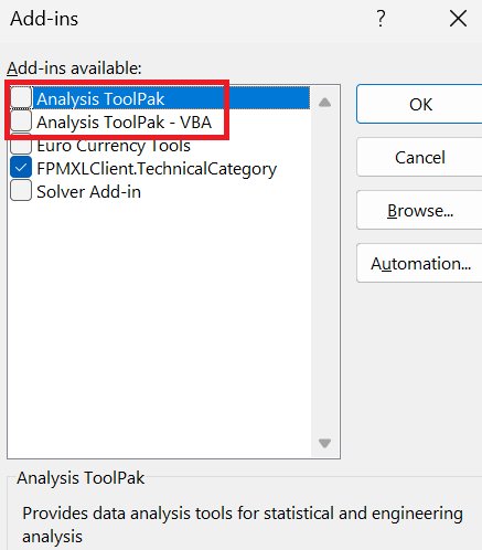
1. Enabling the Data Analysis ToolPak on Windows: select File, then Options, then the Add-Ins category.
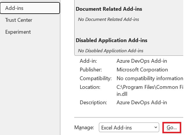
2. In the Manage box, select Excel Add-ins, then select Go.
3. In the Add-Ins box, check Analysis ToolPak and select OK. If Excel says it is not installed, select Yes to install it.
4. On a Mac, open the Tools menu, select Excel Add-ins, and check Analysis ToolPak there.
5. Using the Descriptive Statistics feature: on the Data tab, select Data Analysis, choose Descriptive Statistics and select OK.
6. In the dialog, enter your data column as the input range, choose where the report should go, and turn on the summary statistics option.
7. Select OK and read the mean, median and mode in the report table Excel creates.

The tool works on one worksheet at a time. On grouped worksheets, results appear only on the first sheet, so run it again on each of the others.

Method 3: Manual calculation with sorting and counting

This method shows the working, which suits homework, teaching, or checking a formula result you do not trust.

1. Select a cell in the data column, then on the Data tab, in the Sort & Filter group, select Sort Smallest to Largest.
2. Calculating the mean: type =SUM(A2:A11)/COUNT(A2:A11) in an empty cell. The sample gives 800 / 10 = 80.
3. Calculating the median: with an odd count, read the middle cell of the sorted list. With an even count, average the two middle cells; for ten scores that is the 5th and 6th values, (81 + 85) / 2 = 83.
4. Calculating the mode: in B2, type =COUNTIF($A$2:$A$11,A2) and press Enter.
5. Drag the fill handle from B2 down to B11 to count how often each value occurs.
6. Find the highest count in column B. The value beside it is the mode; in the sample, 85 has a count of 3.

If the sort puts some numbers in an odd order, the column mixes numbers stored as numbers with numbers stored as text. Convert them all to numbers and sort again.

How to check Excel mean, median and mode results

1. Select the data cells, for example A2 to A11.
2. Read the status bar at the bottom of the Excel window. It shows Average, Count and Sum for the selection.
3. Compare the status bar Average with your AVERAGE cell. They must match exactly.
4. Check that Count equals the number of values you expect. A lower count means some cells hold text, not numbers.
5. Confirm the mode by sorting a copy of the data: the mode is the value with the longest run of repeats.
6. Check the median against the sorted list: half the values sit on each side of it.

Visualizing mean and median results in an Excel chart

A box and whisker chart shows how the data spreads into quartiles, with a marker for the mean and separate points for outliers. It makes the gap between mean and median visible at a glance.

1. Select the data column, or several columns to compare groups side by side.
2. Select Insert > Insert Statistic Chart > Box and Whisker.
3. Right-click one of the boxes and select Format Data Series.
4. Under Series Options, turn on Show mean markers to mark the mean on each box.
5. Under Quartile Calculation, choose Inclusive median or Exclusive median to set how the median is handled for an odd count.
6. Use the Chart Design and Format tabs to add a title and change colours.

Best practices and tips for Excel averages, medians and modes

Tip	Why it matters
Use absolute references such as $A$2:$A$11 in COUNTIF before filling down	Relative references shift row by row and count the wrong cells
Leave blanks blank instead of typing 0	Zeros are included in every calculation; empty cells are ignored
Prefer MODE.SNGL and MODE.MULT over MODE	MODE is kept only for compatibility and may be removed
Report the median for skewed data	One very large value moves the mean but barely moves the median
Wrap MODE in IFERROR when duplicates are not guaranteed, for example =IFERROR(MODE.SNGL(A2:A11),"No mode")	A list with no repeated values returns #N/A
Use AVERAGEIF or AVERAGEIFS for a conditional mean	They average only the rows that meet your criteria

Advanced tips: dynamic formulas and automation

In Microsoft 365, MODE.MULT is a dynamic array formula: it returns as many results as there are modes and resizes itself when the data changes. MODE.MULT returns a vertical list, so wrap it in TRANSPOSE when the results must run across a row.

=TRANSPOSE(MODE.MULT(A2:A13))

MODE.MULT finds every value that ties for the highest frequency, and TRANSPOSE turns the vertical list into a horizontal one that spills to the right.

You should see: With 1, 2 and 3 each appearing three times in A2:A13, the cell shows 1 and the two cells to its right show 2 and 3.

To include new rows automatically, point the formulas at a whole column, such as =AVERAGE(A:A). A text header in A1 is ignored, but anything else typed in that column below the data is counted.

Legacy Ctrl + Shift + Enter array formulas still work for compatibility, but Microsoft advises converting them to dynamic array formulas.

Practical applications and use cases for mean, median and mode in Excel

Data	Most useful measure	Reason
Class test scores	Mean and median together	A gap between them shows a few very high or very low scores
Salaries or house prices	Median	A handful of very large values inflates the mean
Shoe or clothing sizes sold	Mode	Stock planning needs the most common size, not an average size
Daily sales totals	Mean	Values are fairly even, and the mean multiplies back to a total
Survey answers on a 1 to 5 scale	Mode and median	The scale is ordered, but an average like 3.4 is not a real answer
Order quantities with counts per value	Weighted mean with SUMPRODUCT	Each value must count as many times as it occurred

Fix Excel MODE, MEDIAN and AVERAGE errors

MODE.SNGL or MODE.MULT returns #N/A

No value appears more than once in the range, so there is no mode.

1. Sort the data and confirm that no value repeats.
2. Report that the data has no mode, or wrap the formula: =IFERROR(MODE.SNGL(A2:A11),"No mode").

The Data Analysis button is missing from the Data tab

The Analysis ToolPak add-in is not loaded.

1. Select File > Options > Add-Ins.
2. Set Manage to Excel Add-ins and select Go.
3. Check Analysis ToolPak and select OK. If it is not listed, select Browse to locate it.

MODE.MULT shows #SPILL!

Cells below the formula already hold data, so the results have nowhere to spill.

1. Select the formula cell to see the dashed outline of the spill range.
2. Clear or move whatever sits inside that outline, and the results appear.

The mean or median looks wrong

Some values are stored as text and skipped, or zeros stand in for missing entries.

1. Select the data and compare the status bar Count with the number of entries.
2. Convert text-formatted numbers to numbers and sort again.
3. Replace placeholder zeros with blank cells.

Excel mean, median and mode FAQ

How do you find mean, median and mode in Excel?

Use three formulas on the same range: =AVERAGE(A2:A11) for the mean, =MEDIAN(A2:A11) for the median and =MODE.SNGL(A2:A11) for the mode. Replace A2:A11 with your own cells. Use MODE.MULT instead when several values tie for most frequent.

How do you find mean, median, mode and range in Excel?

Add a fourth formula, =MAX(A2:A11)-MIN(A2:A11), next to AVERAGE, MEDIAN and MODE.SNGL. The range is the largest value minus the smallest.

How do you calculate mean and median by hand?

Add all the values and divide by how many there are to get the mean. For the median, sort the values and take the middle one; with an even count, average the two middle values. For 2, 3, 3, 5, 7 and 10, the mean is 5 and the median is 4.

How do you determine the median of an even number of values?

Sort the values and average the two in the middle. Excel's MEDIAN function does this automatically, so =MEDIAN(A2:A7) on 1 to 6 returns 3.5, the midpoint between the third and fourth numbers.

What is the difference between mean and median?

The mean is the sum divided by the count, so every value pulls on it. The median is the middle value, so extreme values barely move it. In symmetrical data they are equal; in skewed data such as incomes, the median better describes a typical value.

How do you find the mean, median and mode from a frequency table in Excel?

With values in A2:A4 and counts in B2:B4, use =SUMPRODUCT(A2:A4,B2:B4)/SUM(B2:B4) for the mean. The mode is the value with the highest count. For the median, list every value as many times as its count and use MEDIAN.

How do you find a missing number when the mean is given?

Multiply the mean by the total number of values to get the required sum, then subtract the sum of the known values. In Excel, =mean*count-SUM(A2:A10) gives the missing value directly once you replace mean and count with your figures.

Is there a quick calculator for mean in Excel without a formula?

Yes. Select the numbers and read the status bar at the bottom of the window, which shows the Average, Count and Sum of the selection. It has no median or mode, so use MEDIAN and MODE.SNGL for those.

Why does Excel show only one mode when there are two?

MODE.SNGL returns only one value, even when several tie. Use =MODE.MULT(A2:A11) to return every mode. In Microsoft 365 the results spill down automatically; in older versions, enter it with Ctrl + Shift + Enter across several cells.