How to calculate inverse matrix in Excel (3 ways)

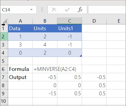
Type =MINVERSE(A2:C4) in an empty cell, using your own square range, and press Enter to calculate the inverse matrix in Excel.

This guide covers the three ways to do it: the MINVERSE function, checking the result with MMULT, and a reusable LAMBDA function, plus a worked example that solves a system of linear equations.

Method 1: Calculating the inverse matrix using MINVERSE

MINVERSE works in Excel for Microsoft 365, Excel 2024, 2021, 2019 and 2016, on Windows and Mac. The examples below use the 3×3 matrix 2, 1, 1 / 1, 3, 2 / 1, 0, 0 in cells A2:C4.

1. Enter your matrix in a square block of cells, such as A2:C4, with a number in every cell and no blanks.
2. Click an empty cell that has the same number of free rows and columns to its right and below, such as E2.
3. Type =MINVERSE(A2:C4).
4. In current Microsoft 365, press Enter. The inverse spills into E2:G4 automatically.
5. In other versions, first select the whole output range E2:G4, type the formula, and press Ctrl + Shift + Enter. Excel wraps the formula in curly brackets.
6. Read the result. For the example matrix, the inverse is 0, 0, 1 / -2, 1, 3 / 3, -1, -5.

If you press plain Enter in a version without dynamic arrays, Excel returns only one value instead of the full matrix. Select the output range and confirm with Ctrl + Shift + Enter to fix that.

Which inverse matrix method fits your Excel version?

The three methods do different jobs. One calculates the inverse, one proves it, and one packages it as a named function you can reuse.

Your situation	Use this	Excel version needed
You need the inverse of one square matrix	Method 1: MINVERSE	Microsoft 365, 2024, 2021, 2019 or 2016
You want proof the inverse is correct	Method 2: MMULT of the matrix and its inverse	Same as MINVERSE
You invert many matrices and want a named function with a singular-matrix check	Method 3: dynamic arrays with LAMBDA	Microsoft 365 or Excel 2024, Windows or Mac
You need to solve a set of linear equations	MMULT(MINVERSE(A), b) from the practical example below	Microsoft 365, 2024, 2021, 2019 or 2016

Understanding the inverse of a matrix

The inverse of a square matrix A is the matrix that, multiplied by A, gives the identity matrix. The identity matrix has 1 on its diagonal and 0 everywhere else.

Only square matrices with a determinant other than 0 have an inverse. Inverse matrices, like determinants, are mainly used to solve systems of equations with several variables.

Term	What it means	Excel function
Square matrix	Same number of rows and columns, such as 2×2 or 3×3	Any range like A2:C4
Determinant	A single number derived from the matrix; 0 means no inverse exists	MDETERM(A2:C4)
Inverse matrix	The matrix that returns the identity matrix when multiplied by the original	MINVERSE(A2:C4)
Identity (unit) matrix	1 on the diagonal, 0 everywhere else	MUNIT(3) for a 3×3
Matrix product	Rows of the first matrix times columns of the second	MMULT(array1, array2)
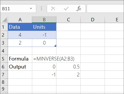
2×2 inverse formula	For a matrix a, b / c, d: d/(ad-bc), -b/(ad-bc) / -c/(ad-bc), a/(ad-bc)	MINVERSE applies this for you

Check the determinant with MDETERM before you invert

A matrix with a determinant of 0 is singular and cannot be inverted. Checking first tells you whether a #NUM! error is a data problem or a formula problem.

1. Click an empty cell, such as I7.
2. Type =MDETERM(A2:C4) and press Enter.
3. Read the result. The example matrix returns -1, so it has an inverse.
4. If the result is 0, or a tiny number such as 1E-16, treat the matrix as singular and check your input values.

MDETERM is accurate to about 16 digits, so the determinant of a singular matrix can come back as a value like 1E-16 instead of exactly 0.

Method 2: Validating the results using MMULT

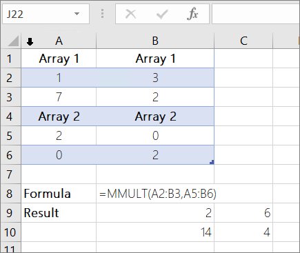
Multiply the original matrix by its inverse. If the inverse is correct, the product is the identity matrix.

1. Click an empty cell with three free rows and columns, such as A7.
2. Type =MMULT(A2:C4,E2:G4) to multiply the original matrix by the inverse.
3. Press Enter in current Microsoft 365, or select A7:C9 first and press Ctrl + Shift + Enter in other versions.
4. Check the result. The diagonal should read 1 and every other cell 0.
5. If you see values such as 2.2E-16 instead of 0, wrap the formula in ROUND: =ROUND(MMULT(A2:C4,E2:G4),10).

MMULT needs the column count of the first array to match the row count of the second. A square matrix and its inverse always meet that rule.

Method 3: Advanced techniques using dynamic arrays and LAMBDA (Excel 365/Excel 2024)

In Microsoft 365 and Excel 2024, LAMBDA turns the inverse calculation into a named function, such as MATINV, that any cell in the workbook can call. This custom function also returns a clear message for a singular matrix instead of #NUM!.

1. Test the formula in a cell first: =LAMBDA(m, IF(ABS(MDETERM(m))<1E-12, "Singular matrix", MINVERSE(m)))(A2:C4). It should spill the same inverse as Method 1.
2. In Excel for Windows, select Formulas > Name Manager, then select New. In Excel for Mac, select Formulas > Define Name.
3. In Name, type MATINV.
4. Leave Scope as Workbook, and add a short Comment such as "Returns the inverse of a square matrix".
5. In Refers to, paste =LAMBDA(m, IF(ABS(MDETERM(m))<1E-12, "Singular matrix", MINVERSE(m))).
6. Select OK, then Close.
7. Type =MATINV(A2:C4) in any empty cell and press Enter. The inverse spills into the cells below and to the right.

Refer to the whole spilled result with the spill operator, for example =MMULT(A2:C4,E2#). The # reference grows or shrinks with the inverse, so the check from Method 2 keeps working if the matrix size changes.

Practical example: solving a system of linear equations

Take the system 2x + y + z = 7, x + 3y + 2z = 13, and x = 1. In matrix form this is A times [x, y, z] equals b, so [x, y, z] equals the inverse of A times b.

1. Enter the coefficients in A2:C4: 2, 1, 1 in row 2; 1, 3, 2 in row 3; 1, 0, 0 in row 4.
2. Enter the constants 7, 13 and 1 in I2:I4.
3. Click K2 and type =MMULT(MINVERSE(A2:C4),I2:I4).
4. Press Enter in current Microsoft 365, or select K2:K4 first and press Ctrl + Shift + Enter.
5. Read the solution in K2:K4: x = 1, y = 2, z = 3.
6. Check one equation by hand: 2(1) + 2 + 3 = 7.

The order of the arrays matters. MMULT(MINVERSE(A),b) returns the solution, while MMULT(b,MINVERSE(A)) returns #VALUE! because the sizes do not line up.

How to check an Excel inverse matrix is correct in one cell

Method 2 shows the full product. This single formula returns one TRUE or FALSE, which suits a dashboard or a large matrix.

=AND(ROUND(MMULT(A2:C4,MINVERSE(A2:C4)),10)=MUNIT(3))

Multiplies the matrix by its inverse, rounds away floating-point noise, and compares every cell with a 3×3 identity matrix from MUNIT. Change 3 to your matrix size.

You should see: TRUE means the inverse is correct. FALSE, #NUM! or #VALUE! points to one of the issues below.

Handling common issues

Find the error or symptom you see, then apply the fix under it.

MINVERSE returns #NUM!

The matrix is singular: its determinant is 0, so no inverse exists.

1. Run =MDETERM(A2:C4) on the same range.
2. If it returns 0 or a value near 1E-16, look for a row or column that is a multiple or sum of others.
3. Correct the input values, or accept that this system has no unique solution.

MINVERSE or MMULT returns #VALUE!

A cell in the range is empty or holds text, or the range is not square.

1. Check that the range has the same number of rows and columns.
2. Fill every empty cell with a number, using 0 where the value is zero.
3. Remove text, including numbers stored as text, then recalculate.
4. For MMULT, confirm the first array has as many columns as the second has rows.

Only one number appears instead of the whole inverse

The formula was entered as a normal formula in a version without dynamic arrays.

1. Select the full output range, such as E2:G4.
2. Press F2 to edit the formula in the top-left cell.
3. Press Ctrl + Shift + Enter. Curly brackets appear around the formula.

The inverse shows #SPILL!

Cells in the spill range are not blank, are merged, or sit inside an Excel table.

1. Select the cell with #SPILL! to see the dashed spill border.
2. Select the error alert, then Select Obstructing Cells.
3. Delete or move the content, unmerge the cells, or move the formula out of the table.

Results show tiny numbers like 1E-16 instead of 0

MINVERSE is accurate to about 16 digits, so cancellation is not always complete.

1. Wrap the result in ROUND, for example =ROUND(MINVERSE(A2:C4),10).
2. Or format the cells to show fewer decimal places, which changes the display but not the stored value.

You cannot edit or delete part of the inverse

A legacy Ctrl + Shift + Enter array must be changed as one block.

1. Select the whole output range.
2. Edit the formula and confirm with Ctrl + Shift + Enter, or press Delete to clear the full range.
3. In Microsoft 365, edit only the top-left cell of a spilled result; the rest updates with it.

Inverse matrix in Excel FAQ

How do you calculate the inverse of a matrix in Excel?

Use the MINVERSE function. Type =MINVERSE(A2:C4) with your square range and press Enter in current Microsoft 365, where the result spills. In other versions, select an output range the same size as the matrix first, then press Ctrl + Shift + Enter.

How do you calculate the inverse of a 3×3 matrix in Excel?

Enter the nine values in a 3×3 block such as A2:C4, then type =MINVERSE(A2:C4) in a cell with three free rows and columns. The result fills a 3×3 range. Check it with MMULT, which should return 1 on the diagonal and 0 elsewhere.

How do you calculate a matrix inverse in a calculator?

The Windows Calculator app offers Standard, Scientific, Programmer and Date calculation modes but no matrix functions. Use Excel's MINVERSE function instead, which handles any square matrix and lets you check the result with MMULT. For a 2×2 matrix, the formula d/(ad-bc) and its partners also work by hand.

Why does MINVERSE return #NUM! in Excel?

MINVERSE returns #NUM! when the matrix cannot be inverted. That happens when its determinant is 0, which you can confirm with =MDETERM(range). Check for a row or column that duplicates or combines others, since no inverse exists for such a matrix.

Why does MINVERSE return #VALUE!?

MINVERSE returns #VALUE! when any cell in the range is empty or holds text, or when the range does not have the same number of rows and columns. Fill blanks with 0, convert text to numbers, and use a square range.

Can you find the inverse of a non-square matrix in Excel?

No. MINVERSE needs a numeric array with an equal number of rows and columns, and returns #VALUE! for any other shape. A 2×3 or 3×4 range has no standard inverse, so MINVERSE cannot help with it.

How do you find the determinant of a matrix in Excel?

Use =MDETERM(A2:C4) with your square range. It returns a single number. A result of 0, or a tiny value such as 1E-16 caused by rounding, means the matrix is singular and has no inverse.

Does MINVERSE need Ctrl+Shift+Enter?

Only in versions without dynamic arrays. In current Microsoft 365, press Enter and the inverse spills. In other versions, select the output range, type the formula in the top-left cell, and press Ctrl + Shift + Enter; otherwise Excel returns a single value.

How do you solve linear equations with an inverse matrix in Excel?

Put the coefficients in a square range and the constants in a column, then use =MMULT(MINVERSE(A2:C4),I2:I4). The result is the column of unknowns. Keep the inverse first in MMULT, or the sizes will not match.

Bottom line: which Excel inverse matrix method should you use?

Use MINVERSE to calculate the inverse, and confirm it once with MMULT before you rely on it. MINVERSE works in every current Excel version and handles any square matrix. The MMULT check catches singular matrices, text in cells and rounding noise in seconds. Move to a named LAMBDA function only if you run Microsoft 365 or Excel 2024 and invert matrices often.